Get infected
Using systems of differential equations
An incredibly wide range of problems can be modelled using differential equations. These range from nuclear waste behaviour to parasites growing on farmed salmon, and from drug absorption and matoblisation to fluid motion. The example below applies differential equations to an epidemic.In late 2019 a new strain of corona virus, COVID 19, emerged which became pandemic in 2020. Due to its infectious and potentially deadly nature, particularly among the old and those with underlying health issues, many governments implemented control strategies to minimise the impact of the outbreak. A key tool used to plan control approaches was the use of mathematical models. One possible model is the SIR model, so called because it compartmentalises the population into the S group - those that are Susecptible to the disease, the I group - those that have the disease and are Infectious, and the R group - those that have had the disease and are Removed from being considered as they can no longer catch or spread the disease (some call R the recovered group, however, many edpidemics have a non-zero mortaility rate and unfortunately not all recover; R must therefore count recovery and death), see graphic below.
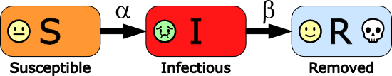
In the above \(\alpha\) is a parameter that describes how infectious the disease is, while \(\beta\) is a parameter that describes how long people are infectious for after they have become infected (they are assumed to be infectious until they recover or they die). A key epidemiological measure, the basic reproduction number, \(R_0\), which essentially describes how many people an infected person will go on to infect, can be derived from these two parameters (see fold-out box below for more details). This value is important because it determines:
- How high the peak number of infections is (will the care system be able to cope with the number of cases?)
- How long it takes for the number of new infections to stop increasing and start decreasing (how long will it take to bring under control?).
- What fraction of the population will be exposed to the disease (how many people will die?).
The SIR model assumes people are "well mixed" so that any susceptible person can be infected by any infected person, and it also assumes that there are no births (any deaths
are grouped with recovered, but now immune people, in the R group). It uses differential equations to describe the evolution of three groups S, I and R, where S, I and R are the number of individuals in each of the three groups
at any given instant, and N is the total population size, \(N = S + I + R \).
The equations that describe how these values change with time are given below.
\begin{aligned} \frac{dS}{dt} &= -\alpha S \frac{I}{N} \\ \\ \frac{dI}{dt} &= \alpha S\frac{I}{N} - \beta I \\ \\ \frac{dR}{dt} &= \beta I \end{aligned} In the above \(\alpha \) is a parameter that describes how infectious the disease is, while \(\beta\) is a parameter that describes how long people are infectious for after they have become infected (they are assumed to be infectious until they recover or they die). Looking at the middle equation for the rate of change of infected individuals it is seen that there are two terms. The first term, \(\alpha S\frac{I}{N}\) states that the number of newly infected people is proportional to the number of susceptible people, S, multiplied by the probabilty of a susceptible person meeting an infected person, \(\frac{I}{N}\). As this represents the number of susceptible people becoming infected per day you should expect an equal number to be lost from the susceptible group, hence the first equation above. The second term in the middle equation states that the number of people being removed from the infectious group is proportional to the number of people infected (essentially if you double the number of infected people you should expect twice as many to get better on any given day). As this is the number of people removed from the infectious group you should expect an equal and opposite change in the number of people in the removed group, hence the third equation above.
The equations above count actual numbers and a total population size, N, is required. Things can be simplified by introducing a change of variables to the following: $$S^* = \frac{S}{N} \quad I^* = \frac{I}{N} \quad R^* = \frac{R}{N} $$ These new variables represent the fraction of the population that are susceptible, infected or removed. Solving for these allows the results to be scaled back to any population size. They also simplify the mathematics. Noting that \(\frac{dS^*}{dS} = \frac{dI^*}{dI} = \frac{dR^*}{dR} = \frac{1}{N} \), the above three equations become \begin{aligned} \frac{dS^*}{dt} &= -\alpha S^* I^* \\ \\ \frac{dI^*}{dt} &= \alpha S^* I^* - \beta I^* \\ \\ \frac{dR^*}{dt} &= \beta I^* \end{aligned} From this point forward it will be assumed that the S, I and R variables represent the fraction of the population in each group and the * will be dropped. Notice how \(\alpha\) and \(\beta\) retain their original definitions.
For an outbreak to be an epidemic, the number of infections must initially be growing. This occurs when \(\frac{dI}{dt} > 0 \), which, in words, reads the rate of change of I with respect to time is positive, i.e. \(I\) is increasing. From the above this occurs when $$\alpha SI - \beta I>0 \Rightarrow \alpha S > \beta . $$ In the early stages of infection there are no people in the R group and only a very small fraction of the population are in the I group. This means that the fraction of the population in the S group is very close to 1. Substituting in to the above, $$\alpha > \beta \Rightarrow R_0 \equiv \frac{\alpha}{\beta} > 1 . $$ The value \(R_0\) is called the basic reproduction number and is a measure of how many people an infected person goes on to infect.
A disease will usually have a non-zero mortality rate, so the total number of deaths is related to the total number of people that have been exposed. An expression for the total fraction of the population that will have been exposed to the disease at the end of the epidemic can be obtained by dividing the expression for \(\frac{dI}{dt}\) by the expression for \(\frac{dS}{dt}\), $$ \frac{\frac{dI}{dt}}{\frac{dS}{dt}} = \frac{dI}{dS} = \frac{\alpha SI - \beta I}{-\alpha SI} = \frac{1}{R_0S} - 1$$ Rearranging and integrating $$\int_{I_0}^{I_\infty} dI = \int_{S_0}^{S_\infty} \left( \frac{1}{R_0S} - 1 \right) dS$$ where \(I_0\) and \(S_0\) are the initial fractions of the population that is infected or susceptible respecitively, and \(I_\infty\) and \(S_\infty\) are the final fractions of the population that is infected or susceptible at the end of the epidmic respecitively. Initially \(I_0 \approx 0\) and \(S_0 \approx 1\), while at the end \(I_\infty = 0\) and \(S_\infty\) is the value of interest. Using these values and evaluating the integral gives $$ 0 = 1 - S_\infty + \frac{ \log_e (S_\infty)}{R_0}. $$ At the end of the epidemic number of people who have been exposed is \(R_\infty = 1 - S_\infty \) (as \(I_\infty = 0\) and \(S + I + R = 1\)). Using this in the above gives an expression for the total fraction of the population that has been exposed during the epidemic: $$ R_0R_\infty + \log_e (1-R_\infty) = 0, \quad \quad 0 \leqslant R_\infty < 1. $$ This equation cannot be solved directly; an iterative method is required. Note, there are generally two roots for this equation, one of which is the trivial solution \(R_\infty = 0\). For the estimated value of \(R_0 = 2.4\) for COVID 19, the above expression is solve when \(R_\infty \approx 0.8786\). This is a little higher than initial "no intervention" values predicted using more sophisticated models, and perhaps hints that the SIR model needs adjustment or refining by possibly adding extra stages.
Looking now at epidemic parameters, the value of \(\alpha \) can be estimated from the intial doubling time for infected individuals, i.e. before people have had a chance to move from the I group to the R group, by looking just at the increase in the number of infected individuals. Using the approximation that \(S \approx 1 \), the equation for the number of infected indivduals is $$ \frac{dI}{dt} \approx \alpha I.$$ The solution of the above is $$I = I_0 e^{\alpha t} $$ For the number of infected people to double from \(I_0\) to \(2I_0\) \begin{aligned} 2I_0 &= I_0 e^{\alpha t} \\ 2 &= e^{\alpha t} \\ \log_e(2) &= \alpha t \end{aligned} For COVID 19 the initial doubling time was reported to be about 3.5 days which gives an estimate of \(\alpha = \frac{\log_e(2)}{3.5} = 0.198 \)
The recovery process in the SIR model assumes a negative exponential distribution with a mean of \( \frac{1}{\beta}\). As \(R_0 = \frac{\alpha}{\beta}\) the estimated initial value of \(R_0 = 2.4\) can be use to give an estimate for \(\beta \) as $$\beta = \frac{\alpha}{R_0} = 0.0825$$ Note, the approach to finding \(\alpha\) and \(\beta\) used here are first approximations only - they should be fine tuned when more data is available!
All the above is under the assumption that initially \(S \approx 1 \), \(I\) is small and \(R=0\). What if \(R > 0\), that is, what if there is already a significant number in the removed group? This could be through obtained immunity, or vaccination. Recall from the above, for an outbreak to be an epidemic, the number of infections must initially be growing. This occurs when \(\frac{dI}{dt} > 0 \), i.e. \(I\) is increasing. From the above this occurs when $$\alpha SI - \beta I>0 \Rightarrow \alpha S > \beta . $$ In the case where \(R > 0\), the approximation \(S \approx 1 \) is replaced by \(S \approx (1-R) \), so that \begin{aligned} \alpha (1-R) &> \beta \end{aligned} Dividing by \(\beta\) and recalling \(R_0 = \frac{\alpha}{\beta}\) \begin{aligned} R_0 (1-R) &> 1 \Rightarrow R < \frac{R_0-1}{R_0}, \end{aligned} for an epidemic to occur. This can be rearranged to ask what minimum value of R is required for an epidemic not to occur. This is simply given when $$ R \geqslant \frac{R_0-1}{R_0} $$ This value is the herd immunity threshold. It states what fraction of a population must be immune for an epidemic not to take off. For \(R_0 = 2.4\), the herd immunity threshold is about 58%. For measles, which has an \(R_0\) in the range of 12 - 18, the herd immunity threshold is about 92 - 94%.
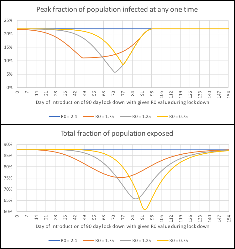
The SIR model uses a set of simultaneous differential equations to model how the number of people in each of the S, I and R groups changes over time for a UK-sized poulation (see fold-out box above for details). These are solved and the results for the number of people in the infectious group are graphed in the interactive element below. This simulation lets the user introduce control measures, such as social isolation, which is intended to reduce the spread of the disease by reducing \(R_0\) during the period for which the action is in place. In this example the lower value of \(R_0\) allowed is 0.75 (this is an arbitrary limit for the sake of example). As this value is less than one it leads to an exponential drop in the number of people in the infectious I group. The time at which restrictions are imposed and lifted is controlled by the two sliders along the bottom. The key things to note are:
- How high the peak number of infections is. If this is too high then the care system will not have enough capacity to cope.
- How long it takes for the number of new infections to stop increasing and start decreasing. The longer this is, the longer a lock-down needs to be in place.
- What fraction of the population will be exposed to the disease. If the mortality rate is 1% and 80% of the population are exposed then for a UK-sized population of about 66.5 million, this translates to about 530,000 deaths.
The model runs for a period of approximately 18 months (30 day months are assumed) with an initial infectious population equivalent to 1,000 people in 66.44 million. It is assumed that after 18 months a suitable vaccine will be available to prevent further spread.