Agents
Using agent-based simulation
Traditionally modelling and simulation has been carried out using differential equations and discrete event simulations, and with good cause as they are very effective methods. Another approach, which has become more popular as computing power grows, is to use an agent-based method, where agents represent individuals or groups of individuals and are allowed to move and react to circumstances. This allows for the capture of complex behaviour such as, for example, details of population movement and allows for reactive behaviour to changes in circumstances.The simulation below is an agent-based representation of a virus epidemic. It considers 25 population centres, each of which is considered "well-mixed", i.e. once an infection takes hold it spreads throughout the population centre. Additionally, people can travel between adjacent population centres, but with a frequency that is much lower than travel within a population centre. In this simplified simulation travel is only possible to adjacent centres along the black lines.
Each population centre is simulated using 10,000 agents and initially 0.1% of one of the centres if infected with the virus. The transmission and recovery characteristics are approximately those of the COVID 19 virus and each agent is characterised as being in one of three groups; the S group - those that are Susecptible to the disease, the I group - those that have the disease and are Infectious, and the R group - those that have had the disease and are Removed from being considered as they can no longer catch or spread the disease (some call R the recovered group, however, many edpidemics have a non-zero mortaility rate and unfortunately not all recover; R must therefore count recovery and death), see graphic below.
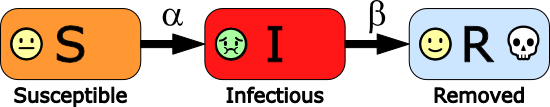
In the above \(\alpha\) is a parameter that describes how infectious the disease is, while \(\beta\) is a parameter that describes how long people are infectious for after they have become infected (they are assumed to be infectious until they recover or they die).
In this simplified agent-based simulation each population centre is simulated with a set of agents, each of which can
meet any other agent in the same population centre with equal probability. For any given agent in the susceptible
group, the probability in any single day of becoming infected is given by the product of the infectiousness of the virus
multiplied by the probability of meeting an infected person per day:
$$ P(S \rightarrow I) = \alpha P(I)$$
If there are \(N\) agents of which \(I\) are infectious, then sampling one agent from the population will yield an infectious agent with probability \(P(I) = \frac{I}{N}\).
Similarly, for any given agent in the susceptible group, the probability in any single day of recovering (or dying) from the infected is given by the recovery rate:
$$ P(I \rightarrow R) = \beta$$
The above is the most basic version of recovery and was chosen so that the simulation behaves in an equivalent way to the
SIR differential equations model (which allows direct comparison of the two approaches
to ensure the agent-based simulation is behaving). An obvious improvement is to more accurately track recovery by drawing
the infectious time from a distribution based on measured data rather than the assumed negative exponential distribution
assumed (which has the obvious drawback that there is a non-zero probability than a patient moves from the infectious group to the
removed group in a single day).
Pseudo-code for an algorithm to perform the basic simulation model described is given below.
There are some gotcha's to consider when using agent-based simulation.
To allow for travel between population centres, the probabily of a susceptible person coming into contact with an infected person from the same population centre \(i\), or from a different population centre \(j\) can be given as: $$ P(S \rightarrow I)^i = \begin{cases} \alpha P(I)^j, & \text{if}\ U \leqslant \gamma \\ \\ \alpha P(I)^i, & \text{otherwise} \\ \end{cases} $$ where U is a uniform random deviate on the interval (0,1] and \(\gamma\) is the probabilty that a person will meet a person from a connected population centre. The pseudo-code above can be adapted to allow for this as follows.
Pseudo-code for an algorithm to perform the basic simulation model described is given below.
// U is a uniform random deviate on the interval (0,1]
For each day:
\(\quad\)For each agent A:
\(\quad \quad\) if A \(\in\) I and U \(\leqslant\) \(\beta\):
\(\quad \quad \quad\) A: I \(\rightarrow\) R
\(\quad \quad\) else if A \(\in\) S:
\(\quad \quad \quad\) B \(\leftarrow \) random agent from population
\(\quad \quad \quad\) if B \(\in\) I and U \(\leqslant\) \(\alpha\):
\(\quad \quad \quad \quad\) A: S \(\rightarrow\) I
There are some gotcha's to consider when using agent-based simulation.
- If the number of agents is small there could be significant variations in results from one simulation run to another and many simulation runs should be made.
- You are at the mercy of random numbers. If you have a small number of agents and only one is initially in the infected group then, depending on the value of \(\beta\), it is possible that many cases will just see the epidemic die out.
- Get a good random number generator!
To allow for travel between population centres, the probabily of a susceptible person coming into contact with an infected person from the same population centre \(i\), or from a different population centre \(j\) can be given as: $$ P(S \rightarrow I)^i = \begin{cases} \alpha P(I)^j, & \text{if}\ U \leqslant \gamma \\ \\ \alpha P(I)^i, & \text{otherwise} \\ \end{cases} $$ where U is a uniform random deviate on the interval (0,1] and \(\gamma\) is the probabilty that a person will meet a person from a connected population centre. The pseudo-code above can be adapted to allow for this as follows.
// U is a uniform random deviate on the interval (0,1]
For each day:
\(\quad\)For each population centre \(i\):
\(\quad\)\(\quad\)For each agent in \(i\), A\(^i\):
\(\quad\)\(\quad \quad\)if A\(^i\) \(\in\) I and U \(\leqslant\) \(\beta\):
\(\quad\)\(\quad \quad \quad\)A\(^i\): I \(\rightarrow\) R
\(\quad\)\(\quad \quad\)else if A\(^i\) \(\in\) S:
\(\quad\)\(\quad \quad \quad\)if U \(\leqslant\) \(\gamma\):
\(\quad\)\(\quad \quad \quad \quad\)j \(\leftarrow \) random connected population centre
\(\quad\)\(\quad \quad \quad \quad\)B \(\leftarrow \) random agent from \(j\)
\(\quad\)\(\quad \quad \quad\)else:
\(\quad\)\(\quad \quad \quad \quad\)B \(\leftarrow \) random agent from population centre \(i\)
\(\quad\)\(\quad \quad \quad\)if B \(\in\) I and U \(\leqslant\) \(\alpha\):
\(\quad\)\(\quad \quad \quad \quad\) A\(^i\): S \(\rightarrow\) I
In the simulation below, select whether there is high or low contact spread between the population centres, then press the start button. Each population centre will follow its own agent-based simulation with occasional population mixing between horizontally and vertically adjacent population centres.
Note, in the simulation below the results are pre-calculated rather than generated in real time. This is because agent-based simulations are typically computationally intensive and generating results at the frame rates they are viewed on this page is not feasible.