Time to queue
Using discrete event simulation
There are many systems where continuous monitoring in time is not an important concern but instead what does matter is when an event occurs that changes the state of the system. One such example is a queue, which could represent, amongst other things:- People arriving at a check-out till to be served in a supermarket.
- Patients waiting for admission, transfer or discharge in a hospital.
- Servers receiveing data requests from clients.
- How long can the queue get? If it gets too long people could abandon the queue and revenue is lost, or there could be issues fitting the number of people in the space available.
- How long will it take from entering the queue to start to get served? Again, if this is too long people may abandon the queue.
- How long will it take to serve all the custemers expected to arrive in the hour? Does the checkout have to stay open longer than necessary?
- How hard will the server be working? Will the staff be over or under utilised?
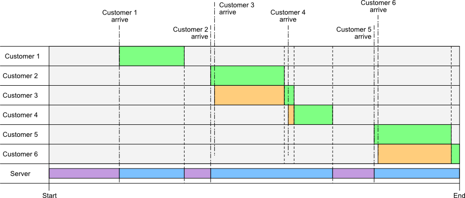
- A customer enters the queue for checkout.
- A customer in the queue starts getting served.
- A customer in the queue finishes getting served and leaves.
The mathematics in this problem is largely based around statistical distributions.
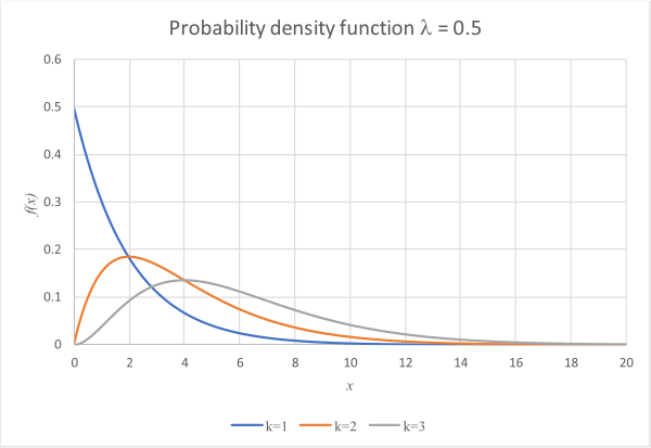
One useful distribution is the Erlang distribution, which is characterised by a shape
parameter, \(k\) and a rate parameter, \(\lambda\). When \(k = 1\), the distribution is an exponential distribution, while with larger values the distribution tends towards a normal distribution. The rate parameter determines
how fast the distribution drops to zero and the location of the maximum when
\(k \geqslant 2\). The larger the value of \(\lambda\), the quicker the distribution drops to zero, and the further to the left the peak value occurs.
$$ f(x;k,\lambda )={\lambda ^{k}x^{k-1}e^{-\lambda x} \over (k-1)!}\quad {\mbox{for }}x,\lambda \geq 0$$
The mean of an Erlang distribution is given by $$Mean \left( f(x;k,\lambda \right) = \frac{k}{\lambda}. $$ The Erlang distribution is very useful in queuing problems. The Erlang distribution with \(k=1\) models the inter-arrival time between customers (which are assumed to be indepedndent events). In this case the mean time between arrivals is \(\frac{1}{\lambda}\), so \(\lambda\) represents the mean number of arrivals per unit time. The probability that exactly \(n\) customers arrive in the unit time is given by the Poisson distribution: $$ f (n;\lambda)= \frac{\lambda ^n e^{-\lambda}}{n!}. $$ As an aside, this distribution also models the number of count events measured by a Geiger counter when detecting ionising radiation from radioactive decay.
An Erlang distribution may also be used to model the time it takes to serve a customer. The distribution with \(k=1\) could be used but this allows for very short service times with reasonably high probabilty. In a customer-service situation this may not be realistic as time will be taken to unload at the checkout and for payment to be taken. To allow for this values of \(k \geqslant 2\) may be used. Recall the mean service time is given by \(\frac{k}{\lambda}\), so \(\frac{\lambda}{k}\) is the mean number of customers served per unit time. In the simulation below, \(k=2\), so to serve an average of \(s\) customers per unit time the Erlang distribution with \(\lambda = 2s\) should be used.
To construct a simulation a method of drawing time intervals from the Erlang distribution is required. For the \(k=1\) case the distribution reduces to the exponential distribution $$ f(x;\lambda ) = \lambda e^{-\lambda x} $$ Integrating this between \(x=0\) and \(x=t\) gives the probability that an event will happen within time t. $$P(event) = \int_{0}^{t} \lambda e^{-\lambda x} dx = 1-e^{-\lambda t}.$$ Rearranging, $$ t = -\frac{1}{\lambda} \ln \left(1 - P(event)\right)$$ If the event occurs at random then \(1-P(event)\) can be replaced by a random uniform deviate, U, on the interval (0,1]. This gives a method for generating random exponentially-spaced times between events as $$ t = -\frac{1}{\lambda} \ln U .$$ For the case where \(k \geqslant 2\) the above is generalised using \(k\) uniform deviates as $$ t = -\frac{1}{\lambda} \ln \prod_{i=1}^{k} U_i .$$
The interactive below uses the results from a discrete event simulation of the checkout queue (coded in Python). The simulation assumptions are
- The initial queue length is zero.
- The mean customer arrival rate is 1 per minute.
- The mean customer service rate is 1.2 per minute.
- The simulation will server 60 customers.
- How long can the queue get?
- How long will it take from entering the queue to start to get served?
- How long will it take to serve all the custemers expected to arrive in the hour?
- How hard will the server be working?
For each of the measurements of interest, the range, mean and median values are displayed. It is also possible to show a set of quantile ranges:
- 25% - 75%, the interquartile range. This is the range of values experienced by the middle 50% of customers.
- 5% - 95%. This is the range of values experienced by the middle 90% of customers.
- 2.5% - 97.2%. This is the range of values experienced by the middle 95% of customers.