Forecasting
Using a Holt-Winters triple exponentially smoothed method
Forecasting is the art of using historical data to predict the future. All forecasting methods use an underlying mathemtaical model, which can range from a straight-line fit for simple cases through to a complex set of differential equations for less simple cases, e.g. predicting the weather. By way of example, consider the following time series data and ask a simple question: can we predict the next three values?
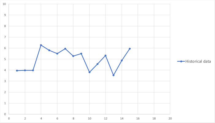 The most simple prediction method is to say the next three points are all equal to the last point in
the data. This is unsatisfactory as the points clearly change through time and the last point
might not be a good representative value.
The most simple prediction method is to say the next three points are all equal to the last point in
the data. This is unsatisfactory as the points clearly change through time and the last point
might not be a good representative value.
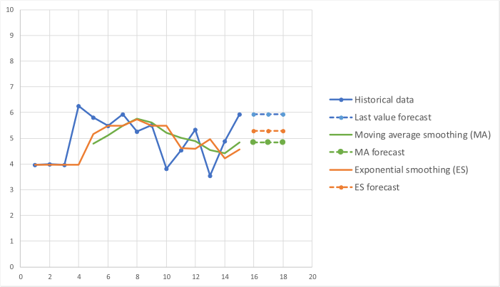
An alternative method is to smooth the data and plot a moving average of the last \(N\) values and use the last average as the estimate \(N\). Moving averages are useful in determining trends in data, but require at least \(N\) points to get started, and count the importance of all data points equally. This may not be appropriate as the most recent data may be deemed to be of higher importance than older data. To allow for this a weighting can be applied so that the most recent points have a higher importance attached to them than points further back in time. One method of doing this is to use exponential smoothing. The advantage of exponential smoothing is that it can be started with a single point (however, generally several points are required for the method to work correctly) and the mathematics are simple to implement.
The graph below shows the result of using each of the three methods above to the data.
 The above is a simple case but time series are not always so accommodating. In general,
a time series of data may be complicated by:
The above is a simple case but time series are not always so accommodating. In general,
a time series of data may be complicated by:- Having an underlying trend of growth or decline.
- Having seasonal effects, e.g. how ice cream sales varies through the year.
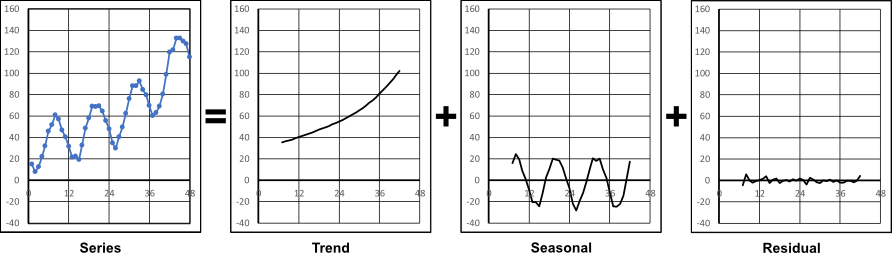 In the above, the components are additive. However, this is not always the case; sometimes
they can be multiplicative. To determine which case applies depends on the data, and a
series decomposition can be performed to evaluate whether additive or multiplicative is
the most appropriate. The Python library statsmodels makes available the function
seasonal_decompose to perform this (or it can be done manually in a spreadsheet).
An example usage is shown below.
In the above, the components are additive. However, this is not always the case; sometimes
they can be multiplicative. To determine which case applies depends on the data, and a
series decomposition can be performed to evaluate whether additive or multiplicative is
the most appropriate. The Python library statsmodels makes available the function
seasonal_decompose to perform this (or it can be done manually in a spreadsheet).
An example usage is shown below.
from statsmodels.tsa.seasonal import seasonal_decompose
import matplotlib as mpl
data=[ ... time series data... ]
print("\nSeasonal decomposition")
sd=seasonal_decompose(data,model='additive',freq=12)
with mpl.rc_context():
mpl.rc("figure",figsize=(12,6))
fig=sd.plot()
import matplotlib as mpl
data=[ ... time series data... ]
print("\nSeasonal decomposition")
sd=seasonal_decompose(data,model='additive',freq=12)
with mpl.rc_context():
mpl.rc("figure",figsize=(12,6))
fig=sd.plot()
Exponential smoothing can also be applied to the above time series, however in this case the smoothing is not only applied to the value, but also to how the value changes with trend, and how it changes with season (month in this case). This is the Holt-Winters method.
Let \(Y_t\) be the actual value of a point in a time series at time \(t\). A forecast for the
value at time \(t+1\), \(F_{t+1}\), can be made using a weighted average of the previous known
values:
$$ F_{t+1}=w_0Y_t+w_1Y_{t-1}+w_2Y_{t-2}+\cdots $$
When \(N\) terms are used and \(w_0 = w_1 = \cdots = w_N = \frac{1}{N}\), the series produces
an \(N\) length backwards moving average. Note, other moving averages such as central or forward moving averages can be constructed by defining where the range of data used falls
with respect to \(t\).
If instead of the above, the form \(w_i=\alpha(1-\alpha)^i\) for some constant \(\alpha\) is used the forcast becomes $$ F_{t+1}=\alpha Y_t+\alpha(1-\alpha)Y_{t-1}+\alpha(1-\alpha)^2Y_{t-2}+\alpha(1-\alpha)^3Y_{t-3}+\cdots $$ Factoring out \(1-\alpha\) from the second terms onwards on the right-hand side gives $$ F_{t+1}=\alpha Y_t+(1-\alpha)(\alpha Y_{t-1}+\alpha(1-\alpha)Y_{t-2}+\alpha(1-\alpha)^2Y_{t-3}+\cdots) $$ But, by definition $$ \alpha Y_{t-1}+\alpha(1-\alpha)Y_{t-2}+\alpha(1-\alpha)^2Y_{t-3}+\cdots = F_{t} $$ So the expression for the forecast simplifies to $$ F_{t+1}=\alpha Y_t+(1-\alpha)F_{t} $$ i.e., the forcast at the next time point is equal to the weighted average of the last time point and the forecast value of the last time point. The weighting factor, \(\alpha\), is found such that it minimises the difference between the known data and the series forecasts for those points using the above induction, subject to \(0 \leqslant \alpha \leqslant 1\). For the simple expontial smoothing example above the value of \(\alpha\) which minimises (in this case) the mean absolute error is found to be \(\alpha=0.521\). A value \(F_1=Y_1\) can be used to initialise the forecast.
The Holt-Winters method expands this exponential smoothing to include an expected level and slope, \(a_t\) and \(b_t\) respectively, to allow for the trend, and a seasonal adjustment, \(s_t\), to allow for seasonal variation. For an additive trend and seasonality, the smoothing is carried out using \begin{aligned} a_t &= \alpha (Y_t - s_{t-p}) + (1-\alpha)(a_{t-1}+b_{t-1}) \\ \\ b_t &= \beta(a_t - a_{t-1})+(1-\beta)b_{t-1} \\ \\ s_t &= \gamma(Y_t - a_t)+(1-\gamma)s_{t-p} \end{aligned} where \(\alpha\), \(\beta\) and \(\gamma\) are the smoothing coefficients for the level, slope and seasonal values respectively, and \(p\) is the period of the seasonal data; 12 in this example. To initialise the series at least one whole seasonal cycle plus an extra value is required, and the values of the forecast for fitting purposes starts at \(F_{p+1}\). The initialisations for \(a_p\), \(b_p\) and \(s\) are \begin{aligned} a_p &=\frac{1}{p}(Y_1+Y_2+ \cdots +Y_p) \\ \\ b_p &= \frac{1}{kp} \sum_{i=1}^{k} \left( Y_{p+i} - Y_{i} \right) \\ \\ s_i &= Y_i - a_p, \quad i=1,2, \cdots , p. \end{aligned}
where \(k\) is the number of data points beyond \(p\) used to initialise \(b_p\). Ideally \(k=p\), so two whole seasonal cycles are used. However, if this is not possible a lower value can be used subject to a minimum value of \(k=1\).
The forecast \(m\) months ahead is given by $$ F_{t+m} = a_t + mb_t + s_{t-p+m}$$ Again, the values of \(\alpha\), \(\beta\) and \(\gamma\) are found that minimises the difference between the known data and the series forecasts for those points using the above induction, subject to \(0 \leqslant \alpha,\beta,\gamma \leqslant 1\), and using \(m=1\).
The equations above are relevant for an additive trend and seasonality. There are other possible combinations, as shown below, each with its own set of equations. The set below is known as the Pegels' classification scheme.
| No trend, no seasonal | No trend, additive seasonal | No trend, multiplicative seasonal |
| Additive trend, no seasonal |
Additive trend, additive seasonal |
Additive trend, multiplicative seasonal |
| Multiplicative trend, no seasonal |
Multiplicative trend, additive seasonal |
Multiplicative trend, multiplicative seasonal |
The interactive element below goes through the steps in constructing a Holt-Winters forecast model and uses it to predict values for the next six months.